First-order kinetics in a CMBR
Environmental engineering
Problem statement
Lets consider 3 continuously mixed batch reactors (CMBRs) where a substance with initial concentration \(C_0\) decays with a first-order rate constant \(k_1\). The parameters for each reactor are listed below:
- CMBR 1: \(C_0\) = 10 mg/L , \(k_1\) = 0.1 s\(^{-1}\)
- CMBR 2: \(C_0\) = 5 mg/L , \(k_1\) = 0.1 s\(^{-1}\)
- CMBR 3: \(C_0\) = 2 mg/L , \(k_1\) = 0.1 s\(^{-1}\)
- Plot the concentration in each reactor as a function of time.
- ¿What is the concentration of the substance in each reactor after 10 sec?
Solution
For a CMBR of constant volume \(V\), the concentration of a substance \(C\) that decays with a first-order rate constant \(k_1\) can be modeled as follows:

\[ \dfrac{dC}{dt}V = k_1 C V \tag{1}\]
Assuming that at time \(t=0\) the concentration of substance is \(C_0\), the previous ordinary differential equation (ODE) has the following analytical solution:
\[ C(t) = C_o e^{-k_1t} \tag{2}\]
Note that, in this case, the concentration in the CMBR is independent of the reactor volume. Lets implement this last equation numerically through a function:
Note that our function receives the initial concentration C0, the first-order decay rate constant k1, and the time array. We can use the same function to model the 3 CMBRs.
Plot of concentration
fig, ax = plt.subplots(figsize=(3,3)) # figure size

time    = linspace(0, 20) # time in sec
k1      = [0.1, 0.1, 0.1] # fist-order decay rate constant (1/s)
C0      = [ 10,  5,  2]   # initial concentrations (mg/L)

for i, k in enumerate(k1):
    Ct = conc(C0[i], k, time)
    col = str(i*0.25)
    ax.plot(time, Ct, color=col, label="$C_0$ = %s mg/L" % C0[i])

ax.axvline(10, color='k', ls=':')
ax.set_xlabel("time [s]")
ax.set_ylabel("concentration [mg/L]")
ax.legend(edgecolor='k')
ax.grid()
plt.show()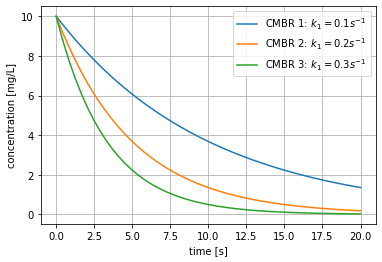
As expected from Equation 2, the concentration of each CMBR decays exponentially as a function of time. We additionally plot a vertical line at \(t=10\) s to visually inspect the concentration at this time.
From Equation 2 we also note that \(1/k_1\) corresponds to the time required to reduce the concentration in the reactor to \(C_0/e\), which is roughly \(\sim\) 37% of the original concentration.
Concentration after 10 sec
We can use our function considering 10 sec as the input time to compute the concentration of the substance.
Follow up questions
- Show that the time it takes a CMBR to reach half of the initial concentration \(t_{1/2} = -\ln(0.5)/k_1\).
- Verify that after a time equal to \(1/k_1\) the concentration in the CMBR is \(C_0/e\).
- How much time is required for the concentration to be exactly zero in each reactor?