from numpy import exp, heaviside as hv

def depth_same(v0, k1, t):
    '''Computes the depth of same particles interface
    '''
    return v0*exp(k1*t)*t

def conc_same(c0, v0, k1, t, h):
    '''Computes the concentration of same particles in a settling jar
    '''
    return c0*hv(h-v0*exp(k1*t)*t, 0)

def conc_many(c0, vi, k1, gi, t, h):
    '''Computes the concentration of many particles ins a settling jar
    '''
    c = 0
    for i, v in enumerate(vi):
        c += conc_same(gi[i]*c0, v, k1, t, h)
return cSettling curve of floccules
Water quality
Problem statement
Determine the settling behavior of particles with a different settling velocities (\(v_i\)), as observed in a settling jar. Assume that initial concentration of particles in the jar is homogeneous (\(C_0\)):
- Develop an expression for the concentration of suspended solids (\(C\)) as a function of depth and time.
- Plot the concentration as a function of time inside the settling jar for particles with \(v_o\) = 1 cm/min.
- Plot the isoconcentration lines for suspended solids removal.
Solution
We assume that particles with identical settling velocity settle solidarily, forming a clear interface between the clarified water and the suspended solids. The depth of this interface can be computed as:
\[ h_i(t) = v_it \qquad \forall i \in \{1,\dots, n\} \tag{1}\]
Note that \(h_i(t)\) is always positive, depends on the particle group with identical settling velocity \(v_i\), and it is measured with respect to a point close to the water surface.
Concentration of suspended solids
By the previous definition, the interface depth can also be used to compute the concentration of suspended solids for each particle group “\(i\)” as a function of time:
\[ C_i(h,t) = \left\{ \begin{aligned} C_{0,i} \qquad h - v_it > 0 \\ 0 \qquad h - v_it \le 0 \end{aligned} \right. \]
The initial concentration \(C_{0,i}\) for each particle group \(i\) can be found through a normalized distribution of particle settling velocities in the suspended solids \(g(v_i)\), which is assumed to be known. Thus,
\[ \begin{align} &C_{0,i} = g(v_i)C_0 \\ &\sum_i g(v_i) = 1 \end{align} \tag{2}\]
Assuming that particles with different settling velocities are indepdent, we can model the total concentration of suspended solids in the settling jar as a summation of the concentration of suspended solids by each particle group “\(i\)”:
\[ \begin{align} &C(h,t) = \sum_i C_{0,i} H(h-v_it) \\ &H(h-v_it) = \left\{ \begin{aligned} 1 \qquad h - v_it > 0\\ 0 \qquad h - v_it \le 0\\ \end{aligned} \right. \end{align} \tag{3}\]
Where \(H(x)\) is the Heaviside step function. Lets compute the concentration through a function:
Plot of suspended solids concentration
We can use our function to compute the concentration in a grid of depth and time for the settling jar. Since we also want to overlay the isoconcentration lines of removal we will annotate the concentration on top of the grid:
from numpy import linspace, meshgrid
from scipy.stats import norm

c0 = 350           # initial concentration mg/L
k1 = 0.3           # kinetic aggregation 1/h

# settling velocities cm/h (slower to higher)
# normalized distribution of particles (slower to higher)
vi = linspace(14, 200, 31)
gi = linspace(norm.pdf(-1.5), norm.pdf(1.5), 31)
gi = gi/gi.sum()

# defining depth and time values
h  = linspace(0, 120, 7)   # depth cm
t  = linspace(0.0, 2.0, 5) # time hours

# computing concentration in grid
xm, ym = meshgrid(t, h)
c      = conc_many(c0, vi, k1, gi, xm, ym)
The function meshgrid of numpy is used to conveniently compute the concentration of suspended solids in the grid. Once computations have been performed we can plot the settling results.
from numpy import arctan2, rad2deg, cumsum
import matplotlib.pyplot as plt

# plotting SS concentration
fig, ax = plt.subplots(figsize=(4,4))
for i in range(len(t)):
    for j in range(1,len(h)-1):
        ax.text(t[i], h[j], '%d'%c[j,i], va='center',
                fontsize=12, ha='center', backgroundcolor='w')

# parameters for isoconcentration removal curves
eff    = ['%d%%'%d for d in 100*cumsum(gi[::-1])][::-1]
eff    = eff[:-17:3]                         # eff subsampling
vs     = vi[:-17:3]                          # vi subsampling
gs     = gi[:-17:3]                          # gi subsampling
delta  = 0.00                                # delta location
xt     = 0.7                                 # x-pos location
yt     = [depth_same(v, k1, xt) for v in vs] # y-pos location
angles = [rad2deg(arctan2(max(v*t),max(t))) for v in vs]

# plotting isoconcentration removal
tnew = linspace(0,2)
for i, v in enumerate(vs):
    ax.plot(tnew, depth_same(v, k1, tnew), lw=1, color='k')
    ax.text(xt+delta, yt[i], eff[i], rotation=angles[i],
            fontsize=14, rotation_mode='anchor',
            transform_rotates_text=True)

# figure decorators
#ax.yaxis.set_tick_params(length=20)
ax.set_yticklabels([])
ax.set_xlim([min(t), max(t)])
ax.set_ylim([max(h), min(h)])
ax.set_xticks(t)
#ax.set_ylabel('depth [cm]')
ax.set_xlabel('tiempo [h]')
ax.grid()
plt.show()
fig.savefig('fig.png', dpi=300)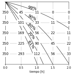
Several observations can be made for the plot:
- The depth is plotted with an inverted axis, to convey a physical meaning to this parameter and to follow the convention for showing settling results.
- The location of isoconcentration removal curves is defined exclusively by the discrete settling velocities.
- The % removal of each isonconcentration curve is defined by the inverse of the cumulative sum of the normalized velocity distribution \(g(v_i)\).
- Note that the curves actually define isoconcentration removal regions, owing to the discrete nature of \(g(v_i)\).
Follow up
- Modify \(v_0\) to achieve 100% particle removal at a depth of 120 cm after 1.5 hours.
- Modify the depth value to show only the first 100 cm depth.
- How would the plot be modified if an additional settling velocity (\(v_1\)) exits for 50% of the particles?