Settling curve of same particles

Water quality

Problem statement

Determine the settling behavior of particles with the samesettling velocity (\(v_0\)), as observed in a settling jar. Assume that initial concentration of particles in the jar is homogeneous (\(C_0\)):

1. Develop an expression for the concentration of suspended solids (\(C\)) as a function of depth and time.
2. Plot the concentration as a function of time inside the settling jar for particles with \(v_o\) = 1 cm/min.
3. Plot the isoconcentration lines for suspended solids removal.

Solution

We assume that the particles settle solidarily, forming a clear interface between the clarified water and the suspended solids. The depth of this interface can be computed as:

\[ h(t) = v_0t \tag{1}\]

Note that \(h(t)\) is always positive, and it is measured with respect to a point close to the water surface.

Concentration of suspended solids

By the previous definition, the interface depth can also be used to compute the concentration of suspended solids as a function of time:

\[ C(h,t) = \left\{ \begin{aligned} C_0 \qquad h - v_0t > 0 \\ 0 \qquad h - v_0t \le 0 \end{aligned} \right. \]

Therefore we can model the concentration of suspended solids in the settling jar as follows:

\[ \begin{align} &C(h,t) = C_0 H(h-v_0t) \\ &H(h-v_0t) = \left\{ \begin{aligned} 1 \qquad h - v_ot > 0\\ 0 \qquad h - v_ot \le 0\\ \end{aligned} \right. \end{align} \tag{2}\]

Where \(H(x)\) is the Heaviside step function. Lets compute the concentration through a function:

from numpy import heaviside as hv

def depth(v0,t):
    '''Computes the depth of suspended solids interface
    '''
    return v0*t

def conc(c0, v0, t, h):
    '''Computes the concentration of solids in a settling jar 
    '''
    return c0*hv(h-v0*t, 0)

Plot of suspended solids concentration

We can use our function to compute the concentration in a grid of depth and time for the settling jar. Since we also want to overlay the isoconcentration lines of removal we will annotate the concentration on top of the grid:

from numpy import linspace, meshgrid

c0 = 10   # initial concentration mg/L
v0 = 60   # settling velocity cm/h

# defining depth and time values
h  = linspace(0, 120, 7)   # depth cm
t  = linspace(0.0, 2.0, 5) # time hours

# computing concentration in grid
xm, ym = meshgrid(t, h)
c      = conc(c0, v0, xm, ym)

The function meshgrid of numpy is used to conveniently compute the concentration of suspended solids in the grid. Once computations have been performed we can plot the settling results.

from numpy import arctan2, rad2deg
import matplotlib.pyplot as plt

# plotting SS concentration
fig, ax = plt.subplots(figsize=(5,5))
for i in range(len(t)):
    for j in range(1,len(h)-1):
        ax.text(t[i], h[j], '%d'%c[j,i], va='center', 
                fontsize=12, ha='center', backgroundcolor='w')

# parameters for isoconcentration removal curve
xt    = 1.1            # x-pos location
yt    = depth(v0, xt)  # y-pos location
delta = 0.05           # delta location
angle = rad2deg(arctan2(max(h),max(t)))

# plotting isoconcentration removal
ax.plot(t, depth(v0, t), lw=2, color='k')
ax.text(xt+delta, yt, '100%', rotation=angle, 
        fontsize=14, rotation_mode='anchor', 
        transform_rotates_text=True)

# figure decorators
ax.yaxis.set_tick_params(length=20)
ax.set_xlim([min(t), max(t)])
ax.set_ylim([max(h), min(h)])
ax.set_xticks(t)
ax.set_ylabel('depth [cm]')
ax.set_xlabel('time [h]')
ax.grid()
plt.show()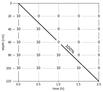

Several observations can be made for the plot:

• The depth is plotted with an inverted axis, to convey a physical meaning to this parameter and to follow the convention for showing settling results.
• Only one isoconcentration removal curve is computed (100%), since a single settling velocity exits. Note however that this line effectively produces 2 regions, one with perfect solids removal and one with no solids removal.
• The slope of the water-solids interface corresponds the settling velocity.

Follow up

1. Modify \(v_0\) to achieve 100% particle removal at a depth of 120 cm after 1.5 hours.
2. Modify the depth value to show only the first 100 cm depth.
3. How would the plot be modified if an additional settling velocity (\(v_1\)) exits for 50% of the particles?