# tracer essay results
# Mp = 1000000 mg
# Q = 150 L/min
# V = 5058 L
# time[min] conc[mg/L]
0 17.943Hydraulic behavior of a reactor
Water quality
Problem statement
You have been commissioned to assess the hydraulic behavior of a reactor built for a continuous mix process. To this end you have performed a tracer test for the reactor, injecting an instantaneous pulse of rodamine with mass \(M_p\) at the inlet of the reactor, and measuring the concentration \(c_p\) at the outlet. The measured results are available in the file tracer_results.txt.
- Plot the tracer concentration at the reactor outlet as a function of time.
- Plot the the exit age distribution \(E(t)\), and the cumulative exit age distribution \(F(t)\):
\[ E(t) = \frac{Q}{M_p} c_p(t) \tag{1}\] \[F(t) = \int_0^t E(t)dt \tag{2}\]
- Compute the Morril index \(T_{90}/T_{10}\).
Solution
Before solving this problem, it is always instructive to first check the data we will be working on. Most plain text files store valuable information in the header, and we often need to check this information to properly read the file.
File checking is often performed directly reading the file with a competent program such as Notepad++. However here we will be reading the first six lines of the file directly with python:
Following our initial check, we recognize that our file contains 2 columns, one for time and one for the tracer concentration. We also note that the header information is identified with the ‘#’ character. Additional valuable information is also provided, so we store it for later use:
Plot of tracer concentration
Once we know the contents of our file, our first task is straightforward: first we read and store the data in the text file, and then we plot it.
We will be reading our data with the loadtxt function of numpy. Since we already know that our file contains 2 columns, we will be unpacking them in 2 arrays. Note that we also pass the ‘#’ character to loadtxt to identify comment lines.
from numpy import loadtxt
import matplotlib.pyplot as plt

# loading data and plotting figure
time, conc = loadtxt(fname, comments='#', unpack=True)
fig, ax    = plt.subplots(figsize=(6,5))
ax.plot(time, conc, lw=2, color='limegreen')

# axes decorations
ax.set_title('Rodamine concentration at the outlet')
ax.set_xlabel('time [s]')
ax.set_ylabel('Concentration [mg/L]')
plt.show()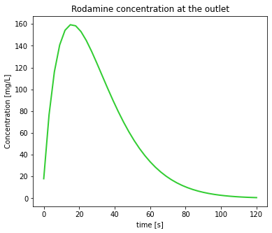
We note that the outlet concentration is not symmetric with respect to time, exhibiting a concentration tail for later times. This is an expected behavior for well mixed reactors.
Plot of distribution metrics
Following Equation 1, computation of the exit age distribution is straightforward. For the case of the cumulative exit age distribution, we need to proceed by numerical integration, in this case using the cumulative integration function cumulative_trapezoid:
\[F(t) = \int_0^t E(t)dt \approx \sum_{i=0}^t E(t) \Delta t_i \]
from scipy.integrate import cumulative_trapezoid
# computing residence time distribution metrics
ead = Q *conc / Mp
fad = cumulative_trapezoid(ead, time,initial=0)

# plotting figures
fig, axes = plt.subplots(1,2, figsize=(12,5))
axes[0].plot(time, ead, lw=2)
axes[1].plot(time, fad, lw=2)

# decorators
axes[0].set_title('Exit age distribution')
axes[0].set_ylabel('E(t) [min$^{-1}$]')
axes[1].set_title('Cumulative exit age distribution')
axes[1].set_ylabel('F(t) [adim]')
for ax in axes:
    ax.set_xlabel('time [min]')
plt.show()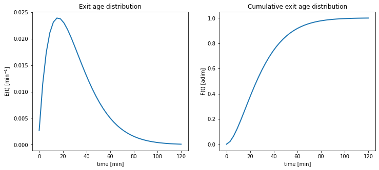
Morril index
To compute \(T_{90}\) and \(T_{10}\) we need to use the cumulative exit age distribution. Here we will create an interpolated function for time as a function of \(F(t)\), in order to precisely compute the required time values.
from scipy.interpolate import interp1d

# computing residence metrics
f     = interp1d(fad, time, kind='cubic')
fracs = [0.1, 0.5, 0.9]
times = f(fracs)

#printing results
for i, val in enumerate(times):
    print('T{0:2.0f} = {1:>4.1f} min'.format(fracs[i]*100, val) )
print('Morril index = {0:1.3f}'.format(times[2]/times[0]) )
T10 = 7.9 min
T50 = 25.5 min
T90 = 56.7 min
Morril index = 7.225Follow up
- Compute the total tracer mass that has leaved the reactor. Compare it with the total pulse mass \(M_p\).
- Compute the experimental residence time \(\hat{\tau}\). Compare it with the theoretical residence time \(\tau\).