from numpy import linspace, exp
import matplotlib.pyplot as plt

def conc_cstr_steady(tau, Cin, k1):
    '''Steady-state concentration in a CSTR with first-order decay
    '''
    return Cin / (1+k1*tau)

def conc_cstr(tau, Cin, C0, k1, time):
    '''Concentration in a CSTR with first-order decay
    '''
    Cinf = conc_cstr_steady(tau, Cin, k1)
return Cinf + (C0 - Cinf) * exp(-time*(1+k1*tau)/tau)First-order kinetics in a CSTR
Environmental engineering
Problem statement
Lets consider a continuously stirred tank reactor (CSTR) where a substance with varying initial concentration \(C_0\) decays with a first-order rate constant \(k_1\). The reactor receives an inflow \(Q\) with a concentration of substance \(C_{in}\), while the outflow equals the inflow. The parameters for each CSTR are the following:
- CSTR 1: \(Q\) = 2 L/s, \(V\)= 20 L, \(C_{in}\) = 12 mg/L, \(C_0\) = 8 mg/L, \(k_1\) = 0.1 s\(^{-1}\)
- CSTR 2: \(Q\) = 2 L/s, \(V\)= 20 L, \(C_{in}\) = 12 mg/L, \(C_0\) = 3 mg/L, \(k_1\) = 0.1 s\(^{-1}\)
- Plot the concentration in each reactor as a function of time.
- Determine the outlfow concentration under steady-state.
Solution
For a CSTR, if the inflow \(Q\) equals the outflow, the net accumulation of water is zero, and therefore the volume \(V\) is constant. In addition, the concentration of a substance \(C\) that decays with a first-order rate constant \(k_1\) can be modeled as follows:

\[ \dfrac{dC}{dt}V = QC_{in} - QC - k_1 C V \tag{1}\]
Since the reactor is continously stirred, the concentration \(C\) inside the reactor equals to outflow concentration. At steady-state (\(dC/dt=0\)) the concentration in the reactor is the following:
\[ C_\infty = \dfrac{C_{in}}{1+k_1 \tau} \tag{2}\]
\[ \tau = \dfrac{V}{Q} \tag{3}\]
Where \(\tau\) corresponds to the hydraulic residence time in the reactor. Note that at steady-state, the concentration of the reaction is proportional to \(C_{in}\), but diluted by a factor of \(1 + k_1 \tau\). Also note that the concentration at steady-state is independent of the initial concentration in the reactor.
Assuming that at time \(t=0\) the concentration of substance in the reactor is \(C_0\), then Equation 1 has the following analytical solution:
\[ C(t) = C_\infty + \left( C_0 - C_\infty \right)\exp \left[-t \left( \dfrac{1 + k_1 \tau}{\tau} \right) \right] \tag{4}\]
Lets implement Equation 2 and Equation 4 numerically through the following functions:
Note that the function conc_cstr() receives the residence time tau, the inflow concentration Cin, the initial concentration in the reactor C0, the first-order decay rate constant k1, and the time array. On the other hand, the function conc_cstr_steady() does not require the time or the initial concentration in the reactor.
Plot of concentration
fig, ax = plt.subplots(figsize=(3,3)) # figure size

time    = linspace(0, 20) # time in sec
Q       = 2               # flow (L/s)
V       = 20              # volume (L)
k1      = 0.1             # first-order decay rate constant (1/s)
Cin     = 12              # inflow concentration (mg/L)
C0      = [8, 3]          # initial concentration (mg/L)
tau     = V / Q           # residence time (s)
ls      = ['-', '--']     # line styles

for i, c0 in enumerate(C0):
    Ct = conc_cstr(tau, Cin, c0, k1, time)
    col = str(i*0.25)
    ax.plot(time, Ct, color='k', ls=ls[i],
            label="$C_0$ = %s (mg/L)" % c0)

ax.axhline(conc_cstr_steady(tau, Cin, k1), color='k', ls=':')
ax.set_xlabel("time [s]")
ax.set_ylabel("concentration [mg/L]")
ax.set_xlim(time.min(), time.max())
ax.legend(edgecolor='k', fontsize=9)
ax.grid()
plt.show()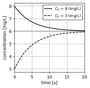
As expected from Equation 4, the concentration of each CSTR approaches exponentally the steady-state concentration as a function of time. We additionally plot an horizontal line at the steady-state concentration, to visually inspect the required time to reach this concentration.
Concentration at steady-state
We can use the function conc_cstr_steady() to determine the concentration of both CSTR at steady-state. Note that in this case only one computation is needed, since the steady-state concentration does not depend on the initial concentration in the reactor:
Follow up questions
- From the mass balance of water in a CSTR, verify that under steady-flow the volume \(V\) remains constant.
- Verify that, for a given inflow with initial concentration \(C_{in}\), a CSTR with \(\tau\) = 2 h and \(k_1\) = 0.1 s\(^{-1}\) produces the same concentration at steady-state than a CSTR with \(\tau\) = 5 h and \(k_1\) = 0.04 s\(^{-1}\).
- Plot the adimensional relation between \(C_\infty/C_{in}\) as a function of \(k \tau\). What is the required value of \(k \tau\) to decrease the inflow concentration in 90% at steady-state?