First-order kinetics in a PFR

Environmental engineering

Author

Marco A. Alsina

Published

January 15, 2026

Problem statement

Lets consider 2 plug flow reactors (PFRs) with constant cross-sectional area \(A\) and length \(L\), where a substance decays with a first-order rate constant \(k_1\). Each reactor receives an inflow \(Q\) with a concentration of substance \(C_{in}\), while the outflow equals the inflow. The parameters for each PFR are the following:

PFR 1: \(Q\) = 5 L/s, \(A\)= 0.2 m\(^2\), \(C_{in}\) = 12 mg/L, \(k_1\) = 0.1 s\(^{-1}\)
PFR 2: \(Q\) = 5 L/s, \(A\)= 0.4 m\(^2\), \(C_{in}\) = 12 mg/L, \(k_1\) = 0.1 s\(^{-1}\)

Compute the mean flow velocity in each reactor.
Plot the concentration in each reactor as a function of position.
Determine the concentration in the reactor at \(x\) = 0.5 m.
Plot the accumulated mass in each reactor as a function of position.

Solution

For a PFR with constant area \(A\) and flow \(Q\), the mean flow velocity is equal to \(v = Q/A\). For an ideal PFR we assume perfect radial mixing, but no mixing along the flow direction. Thus, the concentration inside the reactor varies as a function of position. By considering a moving control volume \(dV = Adx\), located at position \(x=vt\), the concentration of a substance \(C\) that decays with a first-order rate constant \(k_1\) can be modeled as follows:

\[ \dfrac{dC}{dt}dV = QC - QC - k_1 C dV \tag{1}\]

Note that the relation between time and position \(x\) of the control volume is given by the mean flow velocity \(v\):

\[ dt = \dfrac{dx}{v} \tag{2}\]

Replacing Equation 2 in Equation 1 and canceling terms yields the following ordinary differential equation (ODE):

\[ \dfrac{dC}{dx} = -\dfrac{k_1}{v} C \tag{3}\]

Which is analogous to a CMBR reactor with first-rate order kinetics. Assuming that at \(x=0\) the concentration of substance in the reactor is \(C_{in}\), then Equation 3 has the following analytical solution:

\[ C(x) = C_{in} e^{-\frac{k_1}{v}x} \tag{4}\]

Note that the concentration of substance inside the reactor does not depend on the initial concentration in the reactor, since it gets completely washed by the inflow. In addition, the equation allows to compute the concentration inside the reactor regardless of its length \(L\).

Lets implement Equation 4 numerically through the following function:

from numpy import linspace, exp
import matplotlib.pyplot as plt

def conc_pfr(v, Cin, k1, x):
    '''Concentration in a CMBR with first-order decay
    '''
    return Cin * exp(-k1 / v * x)

Note that the function conc_pfr() receives the flow velocity v, the inflow concentration Cin, the first-order decay rate constant k1, and the position array x.

Flow velocity

To compute the flow velocity we simply need to divide the flow \(Q\) by the cross-sectional area \(A\):

Q   = 5               # flow (L/s)
k1  = 0.1             # first-order decay rate constant (1/s)
Cin = 12              # inflow concentration (mg/L)
A   = [0.2, 0.4]      # reactor area (m2)

vel = [Q/(a*1e3) for a in A] # flow velocity (m/s)

for i, v in enumerate(vel):
    print('PFR %i: A = %1.1f m^2; v = %1.2f cm/s'%(i+1, A[i], 100*v) )

PFR 1: A = 0.2 m^2; v = 2.50 cm/s
PFR 2: A = 0.4 m^2; v = 1.25 cm/s

Thus, for a PFR with a given flow \(Q\), the mean flow velocity \(v\) is inversely proportional to the cross-sectional area \(A\).

Plot of concentration

fig, ax = plt.subplots(figsize=(3,3)) # figure size

x   = linspace(0, 1)  # pos in m
ls  = ['-', '--']     # line styles

for i, v in enumerate(vel):
    Cx = conc_pfr(v, Cin, k1, x)
    ax.plot(x, Cx, color='k', ls=ls[i], 
            label="$A$ = %s m$^2$" % A[i])

ax.axvline(0.5, color='k', ls=':')
ax.set_xlabel("position [m]")
ax.set_ylabel("concentration [mg/L]")
ax.set_xlim(x.min(), x.max())
ax.legend(edgecolor='k', fontsize=9)
ax.grid()
plt.show()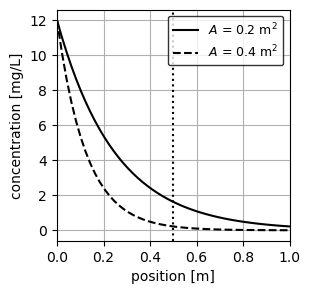

As expected from Equation 4, the concentration of each PFR decays exponentially as a function of position, with the reactor with greater area decaying faster owing to a greater residence time (\(\tau_x=Ax/Q\)). We additionally plot a vertical line at \(x\) = 0.5 m to visually inspect the concentration at this position in the reactor.

Concentration at \(x\) = 0.5 m

We can use the function conc_pfr() to determine the exact concentration of both PFR at \(x\) =0.5 m.

x_eval = 0.5 # m

for i, v in enumerate(vel):
    conc_x = conc_pfr(v, Cin, k1, x_eval)
    print ("PFR %i: C(x=%s[m]): %1.3f [mg/L]" % (i+1, x_eval, conc_x) )

PFR 1: C(x=0.5[m]): 1.624 [mg/L]
PFR 2: C(x=0.5[m]): 0.220 [mg/L]

Accumulated mass of substance in the PFR

To compute the accumulated mass of substance in the reactor we simply need to integrate Equation 4 with respect to a given volume:

\[ M(x) = \int_{0}^{V} C(x)dV = \int_{0}^{x} C_{in}e^{-\frac{k_1}{v}x} A dx \tag{5}\]

\[ M(x) = \dfrac{C_{in}Q}{k_1}\left(1 - e^{-\frac{k_1}{v}x}\right) \tag{6}\]

We implement Equation 6 to plot the mass of substance in the PFR as a function of position:

def mass_pfr(v, Cin, Q, k1, x):
    '''Total mass in a CMBR with first-order decay
    '''
    return Cin*Q*(1- exp(-k1*x/v))/k1

Now lets plot the accumulated mass of substance in each PFR:

fig, ax = plt.subplots(figsize=(3,3)) # figure size

x   = linspace(0, 1)  # pos in m
ls  = ['-', '--']     # line styles

for i, v in enumerate(vel):
    Mx = mass_pfr(v, Cin, Q, k1, x)
    ax.plot(x, Mx/1e3, color='k', ls=ls[i], 
            label="$A$ = %s m$^2$" % A[i])

ax.axvline(0.5, color='k', ls=':')
ax.set_xlabel("position [m]")
ax.set_ylabel("mass [g]")
ax.set_xlim(x.min(), x.max())
ax.legend(edgecolor='k', fontsize=9)
ax.grid()
plt.show()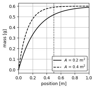

Follow up questions

Verify that when \(L=v/k_1\) the outflow concentration of the PFR is \(C_{in}/e\).
Verify that the maximum accumulated mass of substance in a PFR is \(C_{in}Q/k_1\), regardless of reactor geometry.
Plot the adimensional relation between \(C/C_{in}\) as a function of \(k_1x/v\). What is the required value of \(k_1x/v\) to decrease the inflow concentration in 90%?

Reuse

CC BY-SA 4.0